Abstract
This revisits the 5.2Whales demo, with explicit treatment of the linearization of the system. In scaled variables, we model the populations of krill (\(x_1\)) and baleen whales (\(x_2\)) with the system \[ \begin{aligned} x_1' &= r_1 x_1 (1 - F_1 - x_1 - \nu x_2)\\ x_2' &= r_2 x_2 \left(1 - F_2 - \frac{x_2}{x_1}\right), \end{aligned} \] where \(r_1\), \(r_2\), \(F_1\), \(F_2\) and \(\nu\) are parameters. In this demonstration we take \(F_1 = 0.5\), \(F_2 = 0\), \(\nu = 1\), in which case there are the equilibrium solutions \((x_1,x_2) = (1/4,1/4)\) and \((x_1,x_2) = (1/2,0)\). We consider \(r_1 = r_2 = 2/5\) and graph the solutions to the problem linearized at the equilibrium points along with trajectories found from the nonlinear system.
Use Cases
Lecture: The nonlinear equations may be presented with a minimal explanation of the different terms and used as an example of a system for which critical points and linear behavior there may be found. The demonstrations then graph these behaviors.
Outside of Lecture: Solve the nonlinear system to find the critical points, and then find the linear systems approximating the nonlinear system at each. Show that the behavior that you see from the linear system is consistent with what the demonstrations show.
Model Description
As in 5.2Whales, we consider the interaction between a baleen whale species and its food-source, krill. Baleen whales feed by swimming through seawater in which krill (a crustacean about 5 centimeters long) is found with their mouths open, and then forcing the water out through its baleen, which filters the krill from the water.
We consider the population of krill to be governed by its growth rate, constrained by environmental resources, and reduced by predation and fishing. Similarly, we take the population of whales to increase with a growth rate and be constrained by an environmental limiting factor inversely proportional to the krill population and reduced by predation.
ODE Model
Following 5.2Whales, the krill population \(p_1\) satisfies a modified logistic equation, \[ p_1'(t) = r_1 p_1(t) \left( 1 - \frac{p_1(t)}{K} \right) - C p_1(t) p_2(t) - r_1 F_1 p_1(t), \] where \(p_2\) is the whale population, so that the term \(c p_1(t) p_2(t)\) is the predation term (predation requires an interaction between the populations, and so is proportional to their product), and \(r_1 F_1 p_1(t)\) is the fishing term (the amount of krill caught is proportional to their population, and scaled as a fraction \(F_1\) of their growth rate).
Similarly, if we assume that the carrying capacity for the whale population is inversely proportional to the krill population, as is suggested in [3], we obtain the equation \[ p_2'(t) = r_2 p_2(t) \left( 1 - \frac{p_2(t)}{\alpha p_1(t)} \right) - r_2 F_2 p_2(t) \] for \(p_2\), where the term \(r_2 F_2 p_2(t)\) is again the fishing term. (This model is developed in [3].)
We can nondimensionalize the populations (as in [3], [4], or [5]) by taking \(x_1(t) = p_1(t)/K\) and \(x_2(t) = p_2(t)/(\alpha K)\), that is, by writing the populations as a fraction of their theoretical maxima. Introducing these variables and simplifying, we obtain the system \[ \begin{aligned} x_1' &= r_1 x_1 (1 - F_1 - x_1 - \nu x_2)\\ x_2' &= r_2 x_2 \left(1 - F_2 - \frac{x_2}{x_1}\right), \end{aligned} \] where \(\nu = C\alpha K/r_1\). Solving for the equilibrium solutions, we find there is a single non-zero equilibrium at \[ x_1 = \frac{1 - F_1}{1 + \nu(1 - F_2)},\qquad x_2 = \frac{(1 - F_1)(1 - F_2)}{1 + \nu(1 - F_2)}. \] We will consider solutions near this equilibrium solution. There is a second equilibrium with \(x_2 = 0\), \(x_1 = 1 - F_1 = 1/2\), which we may consider as well.
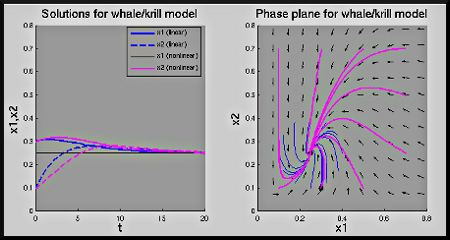
Near the equilibrium solution \((1/4,1/4)\), and taking \(\nu = 1\) (as in [3]), \(r_2 = 0.4\) (which is suggested by [6]), \(F_2 = 0\) (assuming that the whaling ban is actually observed) and the somewhat arbitrarily chosen value \(F_1 = 0.5\), we obtain the linearized system \[ \begin{aligned} u_1' &= -\frac14 r_1 u_1 - \frac14 r_1 u_2\\ u_2' &= \frac25 u_1 - \frac25 u_2, \end{aligned} \] where \(u_1\) and \(u_2\) are the displacements from the equilibrium solution (in the scaled variables, \((1/4, 1/4)\)). We note that \(u_1=0\) and \(u_2=0\) corresponds to \(x_1\) and \(x_2\) being equal to their equlibrium values, \(1/4\). With \(r_1 = 0.4\) as well, the eigenvalues of the coefficient matrix are \(\lambda = -\frac14\pm i\frac{\sqrt{7}}{20}\).
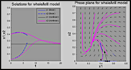
Similarly, near \((1/2, 0)\), we have the coefficient matrix \(\begin{pmatrix} -r_1/2 & -r_1/2\\ 0 & r_2\end{pmatrix}\), and with \(r_1 = r_2 = 0.4\), eigenvalues are \(\lambda = -\frac15, \frac25\).
Matlab Demos
Our demonstrations here show the solutions near each equilibrium solution, and those solutions in the full phase plane.
- Whales_Krill_Coexist.m:
A demonstration that looks at the solutions near the coexistence
point. The solutions to the linearized system are graphed in and
the corresponding trajectory shown in the phase plane, along with a
number of other representative trajectories. These are compared
with the solution to the nonlinear problem, and then numerical
solutions to the nonlinear system are shown for a number of initial
conditions in the phase plane.
Note: also requires the file
plot_localtraj.m.
[show
figure]
- Whales_Krill_Alt.m:
A demonstration that looks at the solutions near the second critical
point. The solutions to the linearized system are graphed in and
the corresponding trajectory shown in the phase plane, along with a
number of other representative trajectories. These are compared
with the solution to the nonlinear problem, and then numerical
solutions to the nonlinear system are shown for a number of initial
conditions in the phase plane.
Note: also requires the files
plot_localtraj.m and
arrow.m
(downloads as a zip file with the Matlab file and license).
[show
figure]
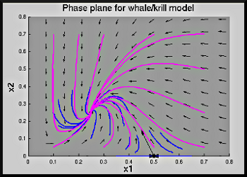
- Whales_Krill_Phase_Plane.m:
A demonstration that looks just at the phase plane. The
trajectories found with the linearized system near each critical
point are graphed in the phase plane, along with a
number of other representative trajectories. Then numerical
solutions to the nonlinear system are shown for a number of initial
conditions in the phase plane.
Note: also requires the files
plot_localtraj.m and
arrow.m
(downloads as a zip file with the Matlab file and license).
[show
figure]
Looking at the Model
Some questions that may be worth considering:
- What do the phase portraits near the equilibrium solutions tell us about the behavior of the system for the full phase plane?
- How do we determine the direction of the spiral trajectories that occur when there are complex eigenvalues?
References
- Wikipedia, Blue Whale. Wikipedia.org. Retrieved on: 23 Oct 2012
- Wikipedia, Fin Whale. Wikipedia.org. Retrieved on: 23 Oct 2012
- May, R.M., Beddington, J.R., Clark, C.W., Holt, S.J. and R.M. Laws (July 1979). "Management of Multispecies Fisheries." Science 205(4403): 267-277.
- Edelstein-Keshet, L. Mathematical Models in Biology, SIAM Classics in Applied Mathematics 46. SIAM, 2005.
- Greenwell, R.N. Whales and Krill: A Mathematical Model, UMAP Module 610. COMAP, 1983.
- Beddington, J.R., and R.M. May (November 1982). "The Harvesting of Interacting Species in a Natural Ecosystem." Scientific American. November 1982: 62-69.
