Math 216 Demonstrations

Model Description

We consider the interaction between a baleen whale species and its food-source, krill. Baleen whales include the blue whale (which can have lengths up to 30 meters; 100 feet)[1] and fin whale (not much smaller, up to 27 meters; 90 feet)[2]. They feed by swimming through seawater in which krill (a crustacean about 5 centimeters long) is found with their mouths open, and then forcing the water out through its baleen, which filters the krill from the water.

We consider the population of krill to be governed by its growth rate, constrained by environmental resources, and reduced by predation and fishing. Similarly, we take the population of whales to increase with a growth rate and be constrained by an environmental limiting factor inversely proportional to the krill population and reduced by predation.

ODE Model

With the assumptions above, the krill population \(p_1\) satisfies a modified logistic equation, \[ p_1'(t) = r_1 p_1(t) \left( 1 - \frac{p_1(t)}{K} \right) - C p_1(t) p_2(t) - r_1 F_1 p_1(t), \] where \(p_2\) is the whale population, so that the term \(c p_1(t) p_2(t)\) is the predation term (predation requires an interaction between the populations, and so is proportional to their product), and \(r_1 F_1 p_1(t)\) is the fishing term (the amount of krill caught is proportional to their population, and scaled as a fraction \(F_1\) of their growth rate).

Similarly, if we assume that the carrying capacity for the whale population is inversely proportional to the krill population, as is suggested in [3], we obtain the equation \[ p_2'(t) = r_2 p_2(t) \left( 1 - \frac{p_2(t)}{\alpha p_1(t)} \right) - r_2 F_2 p_2(t) \] for \(p_2\), where the term \(r_2 F_2 p_2(t)\) is again the fishing term. (This model is developed in [3].)

We can nondimensionalize the populations (as in [3], [4], or [5]) by taking \(x_1(t) = p_1(t)/K\) and \(x_2(t) = p_2(t)/(\alpha K)\), that is, by writing the populations as a fraction of their theoretical maxima. Introducing these variables and simplifying, we obtain the system \[ \begin{aligned} x_1' &= r_1 x_1 (1 - F_1 - x_1 - \nu x_2)\\ x_2' &= r_2 x_2 \left(1 - F_2 - \frac{x_2}{x_1}\right), \end{aligned} \] where \(\nu = C\alpha K/r_1\). Solving for the equilibrium solutions, we find there is a single non-zero equilibrium at \[ x_1 = \frac{1 - F_1}{1 + \nu(1 - F_2)},\qquad x_2 = \frac{(1 - F_1)(1 - F_2)}{1 + \nu(1 - F_2)}. \] We will consider solutions near this equilibrium solution.

Near the equilibrium solution, and taking \(\nu = 1\) (as in [3]), \(r_2 = 0.4\) (which is suggested by [6]), \(F_2 = 0\) (assuming that the whaling ban is actually observed) and the somewhat arbitrarily chosen value \(F_1 = 0.5\), we obtain the linearized system \[ \begin{aligned} u_1' &= -\frac14 r_1 u_1 - \frac14 r_1 u_2\\ u_2' &= \frac25 u_1 - \frac25 u_2, \end{aligned} \] where \(u_1\) and \(u_2\) are the displacements from the equilibrium solution (in the scaled variables, \((1/4, 1/4)\)).[7] We note that \(u_1=0\) and \(u_2=0\) corresponds to \(x_1\) and \(x_2\) being equal to their equlibrium values, \(1/4\).

We consider this last system in this demonstration. As a guess for \(r_1\) we might pick values of 0.3 or greater. Of specific interest are:

• \(r_1 = 1/3\), for which the eigenvalues and eigenvectors of the coefficient matrix are \(\lambda = \frac{1}{120}(-29\pm i\sqrt{119})\) and \(\mathbf{v} = \begin{pmatrix} 19\pm\sqrt{119}\\ 48 \end{pmatrix}\);
• \(r_1 = 0.335\), for which \(\lambda\approx \frac14\pm i\frac1{11}\) and \(\mathbf{v} \approx \begin{pmatrix} \frac25\pm i\frac14\\ 1\end{pmatrix}\); and
• \(r_1 = 4/3\), for which \(\lambda = -\frac{11}{30}\pm i\frac{\sqrt{119}}{30} \approx -\frac13\pm i\frac13\) and \(\mathbf{v} = \begin{pmatrix} 1\pm i\sqrt{119}\\ 12\end{pmatrix}\approx \begin{pmatrix} 1\pm 11 i\\ 12\end{pmatrix}\).

It is also worth noting that if \(r_1 = 4/15\), we have \(\lambda = -4/15\) and \(-1/5\), with \(\mathbf{v} = \begin{pmatrix} 1 & 3\end{pmatrix}^T\) and \(\begin{pmatrix} 1 & 2 \end{pmatrix}^T\).

Matlab Demos

Our demonstration here graphs the solution to this system. (Note that it would not be necessary to do the full derivation of the linearized system to use this model; the linear system could be introduced as a model of the displacements from the equilibrium for the model.)

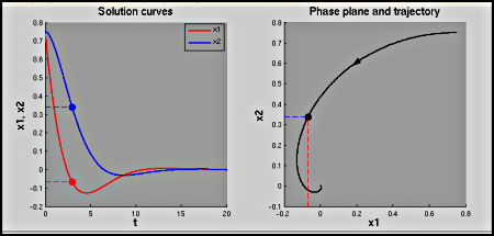
• Whale_Krill_Model.m: A demonstration that graphs the exact solution to the system of two equations. The solution is obtained by finding the eigenvalues and eigenvectors, and then solving for the constants. A configuration parameter show_phase_plane determines whether we graph only the solution, or the solution and trajectory in the phase plane. If the phase plane is shown, the configuration parameters include_pause determines whether there is a pause between graphing the solution and the phase plane, and show_point determines whether a point is shown on the solution curve and trajectory to illustrate the connection between the two. Note: also requires the file arrow.m (downloads as a zip file with the Matlab file and license). [show figure] (no phase plane)
  
  [show figure] (with phase plane)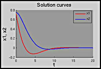
  

Looking at the Model

Some questions that may be worth considering:

• What does our result here say about the stability of the equilibrium solution?
• The default initial condition for the demonstration is \((3/4,3/4)\). What does this mean about \(x_1\) and \(x_2\)?
• How do we determine the direction of the trajectory in the phase plane?

References

1. Wikipedia, Blue Whale. Wikipedia.org. Retrieved on: 23 Oct 2012
2. Wikipedia, Fin Whale. Wikipedia.org. Retrieved on: 23 Oct 2012
3. May, R.M., Beddington, J.R., Clark, C.W., Holt, S.J. and R.M. Laws (July 1979). "Management of Multispecies Fisheries." Science 205(4403): 267-277.
4. Edelstein-Keshet, L. Mathematical Models in Biology, SIAM Classics in Applied Mathematics 46. SIAM, 2005.
5. Greenwell, R.N. Whales and Krill: A Mathematical Model, UMAP Module 610. COMAP, 1983.
6. Beddington, J.R., and R.M. May (November 1982). "The Harvesting of Interacting Species in a Natural Ecosystem." Scientific American. November 1982: 62-69.
7. The linearization proceeds as expected; with \(x_1' = G\) and \(x_2' = H\), the displacement vector \(\mathbf{u}\) satisfies \(\mathbf{u}' = \mathbf{J}(x_{1e}, x_{2e})\mathbf{u}\), where \(\mathbf{J} = \begin{pmatrix} G_{x_1} & G_{x_2}\\ H_{x_1} & H_{x_2}\end{pmatrix}\) is the Jacobian of the system and \(x_{1e}\) and \(x_{2e}\) are the equilibrium values of \(x_1\) and \(x_2\). Here \(G = r_1 x_1 (1 - F_1 - x_1 - \nu x_2)\) and \(H = r_2 x_2 \left(1 - F_2 - \frac{x_2}{x_1}\right)\). Differentiating and plugging in produces the indicated system.