Math 216 Demonstrations

Model Description

As noted in demonstration 4_3Lead, lead has been and continues to be a component in a large number of objects in our environment, and is a neurotoxin.[1] Lead from the environment may enter the body through inhalation or ingestion; in either case, it ends up in the bloodstream and from there may move into the tissues and bones. This behavior is captured by a three-compartment model, as shown below.

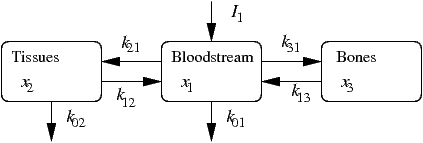
Here lead enters the bloodstream at a rate \(I\), resulting in amounts \(x_1\), \(x_2\) and \(x_3\) in the bloodstream, tissues and bones, and is transferred to compartment \(i\) from compartment \(j\) at a rate \(k_{ij}\). Lead is filtered out of the bloodstream by the kidneys and lost from the tissues into the hair and through tissue loss.

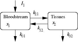
As noted below, the transfer rate into and out of the bones (\(x_3\)) is low, so we might consider that to be zero, reducing the problem to a two-compartment model, as suggested in the figure below.

ODE Model

Assuming that all transfers between and out of the compartments indicated above are proportional to the amount of the lead present there as suggested above, the three compartment model yields the linear system \[ \begin{aligned} x_1'(t) &= -(k_{01} + k_{21} + k_{31})\, x_1(t) + k_{12}\,x_2(t) + k_{13}\,x_3(t) + I_1\\ x_2'(t) &= k_{21}\,x_1(t) - (k_{02} + k_{12})\, x_2(t)\\ x_3'(t) &= k_{31}\,x_1(t) - k_{13}\,x_3(t). \end{aligned} \] with initial condition \(x_1(0) = I_{01}\), \(x_2(0) = I_{02}\) and \(x_3(0) = I_{03}\).

(This model was considered in [2] and expanded on in [3], and is described in [4].) In [3] the values \( I_1 = 49.3 \), \(k_{01} = 0.0211\), \(k_{21} = 0.0111\), \(k_{31} = 0.0039\), \(k_{02} = 0.0162\), \(k_{12} = 0.0124\), and \(k_{13} = 0.000035\) are given for a controlled experiment in which lead was introduced into a male volunteer's diet. Plugging these into the system, we have \[ \begin{aligned} x_1' &= -0.0361 x_1 + 0.0124 x_2 + 0.000035 x_3 + 49.3\\ x_2' &= 0.0111 x_1 - 0.0286 x_2\\ x_3' &= 0.0039 x_1 - 0.000035 x_3. \end{aligned} \] Noting that transfers to and from the third compartment are much smaller than those between the first two, we may choose to ignore that, reducing our problem to a system of two equations, \[ \begin{aligned} x_1' &= -0.0361 x_1 + 0.0124 x_2 + 49.3\\ x_2' &= 0.0111 x_1 - 0.0286 x_2. \end{aligned} \] Let's rescale time to be in years, not days: then \(\frac{d}{dt}_{\,(days)} = \frac1{365}\frac{d}{dt}_{\,(years)}\)[5], so that this becomes \[ \begin{aligned} x_1' &= -13.2 x_1 + 4.5 x_2 + 18,000\\ x_2' &= 4.1 x_1 - 10.4 x_2. \end{aligned} \] If we skew these a little and drop the forcing term, we get the system \[ \begin{aligned} x_1' &= -15 x_1 + 4 x_2 \\ x_2' &= 3 x_1 - 11 x_2, \end{aligned}\] for which the coefficient matrix has eigenvalues \(\lambda = -17, -9\) with corresponding eigenvectors \(\begin{pmatrix} -2\\ 1 \end{pmatrix}\) and \(\begin{pmatrix} 2\\ 3 \end{pmatrix}\). We consider this system, with initial conditions picked to be at the equilibrium values for \(x_1\) and \(x_2\) when the forcing is present, \(x_1(0) = 1300\), \(x_2(0) = 500\).

Matlab Demos

Our demonstration here graphs the solution to this system.

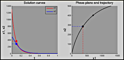
• Lead_Model.m: A demonstration that graphs the exact solution to the system of two equations. The solution is obtained by finding the eigenvalues and eigenvectors, and then solving for the constants. A configuration parameter show_phase_plane determines whether we graph only the solution, or the solution and trajectory in the phase plane. If the phase plane is shown, the configuration parameters include_pause determines whether there is a pause between graphing the solution and the phase plane, and show_point determines whether a point is shown on the solution curve and trajectory to illustrate the connection between the two. Note: also requires the file arrow.m (downloads as a zip file with the Matlab file and license). [show figure] (no phase plane)
  
  [show figure] (with phase plane)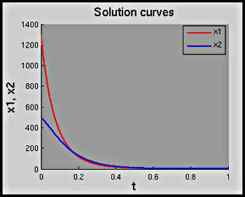
  

Looking at the Model

Some questions that may be worth considering:

• How do we find the equilibrium solutions?
• How are the eigenvectors—in particular, the vector \(\mathbf{v} = \begin{pmatrix} 2\\ 3 \end{pmatrix}\)—visible in the graph of the trajectory?

References

1. Agency for Toxic Substances and Disease Registry (August 2007). ToxFAQs for Lead. Center for Disease Control. Retrieved on: 22 Oct, 2012.
2. Rabinovitz, M.B., Wetherill, G.W., and J.D. Kopple (November 1973). "Lead Metabolism in the Normal Human: Stable Isotope Studies." Science. 182(4113): 725-727.
3. Batschelet, E., Brand, L. and A. Steiner (1979). "On the Kinetics of Lead in the Human Body." Journal of Mathematical Biology 8:15-23.
4. Borelli, R.L. and C.S. Coleman. Differential Equations, a Modeling Perspective, 2nd ed. New York:Wiley, 2004.
5. Let \(s\) be time measured in years. Then \(t = 365 s\) (that is, when \(s = 1\), \(t = 365\)), and we have by the chain rule \(\frac{d}{dt} = \frac{ds}{dt}\times\frac{d}{ds} = \frac{1}{365}\frac{d}{ds}\).