Abstract
We continue analysis of the skydiver model of the 2_3Skydiver demonstration, applying the improved Euler and Runge Kutta methods. Again, the discontinuity in the resistance term provides for a discernable deviation between the numerical methods and between their approximations and the exact solution.
Use Cases
Lecture: It is probably instructive to work a few steps of the improved Euler method to see how it compares with the Euler calculations. It may or may not be useful to similarly work steps of RK. The demonstrations show the difference in the numerical methods, and in their errors.
Outside of Lecture Find the first four approximations to the solution to the initial value problem with the improved Euler's method and \(h=0.6\). Check that your solution matches the values shown in the demonstration, and that you understand the errors illustrated there. Work out the first three steps of the approximation to the solution to the initial value problem using the Runge Kutta method and \(h=0.6\).
Model Description
We again model the velocity of a skydiver by considering her/his motion in two phases, as indicated in 2_3Skydiver, giving the model \[ \frac{dv}{dt} = -g + F_R, \] where \(g\) is the acceleration due to gravity and \(F_R\) is the piecewise defined force of air resistance divided by the mass of the skydiver. We take \[ F_R = \begin{cases} k_1\,v^2 & \mbox{before deployment}\\ -k_2\,v & \mbox{after deployment}. \end{cases} \]
As before, we note that here we take upwards to be the positive direction, so that the force of gravity pulls in the negative direction and \(F_R > 0\) opposes that motion.
ODE Model
Using data from [1], we have (as described in 2_3Skydiver) \[ \frac{dv}{dt} = -32.2 + \begin{cases} 0.00104\,v^2 & \mbox{before deployment}\\ -2.01\,v & \mbox{after deployment} \end{cases}. \] We take \(v(0) = 0\).
Euler's, the improved Euler and Runge Kutta methods are applied in a straightforward manner.
Matlab Demos
We consider a number of Matlab demos for this. These require the file arrow.m (downloads as a zip file with the Matlab file and license) to be in the same directory as the demonstration file, or in the Matlab path.
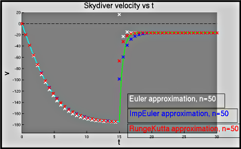
- Skydiver_Numerical_Plot.m:
A very simple demo that just graphs the exact solution and numerical
approximations. In the configuration section of the file one can
specify whether to include the Runge-Kutta method, and whether to
insert a pause between graphs.
[show
figure]
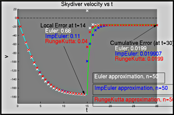
- Skydiver_Numerical_Methods.m:
A demonstration that first graphs the exact solution to the ODE,
pauses, and then, with subsequent pauses, shows the Euler, Improved
Euler and Runge-Kutta approximations; then the local error at a
point, and finally the cumulative error. (Though the latter isn't
very useful, as it is uniformly small.) In the configuration
section of the file one can specify whether to include the
Runge-Kutta method.
[show
figure]
Looking at the Model
Some questions that may be worth considering:
- For each of the methods, how can we predict the number of steps needed to obtain a given level of accuracy?
- Why is the cumulative error for this model and these approximations so similar? In what cases would this not be the case?
- How do the methods' abilities to deal with the discontinuity in the differential equation differ? What does the behavior of the methods at the discontinuity suggest about how other (better, for this type of equation) numerical methods might have to work?
