Abstract
We consider the skydiver model of the 2_3Skydiver demonstration. Euler's method is easily applied, remembering to change the iteration formula when we pass the deployment time. Because of the discontinuity in the resistance, there is an interesting large error immediately after parachute deployment, which allows us to illustrate how the local and cumulative errors in the approximation may differ.
Use Cases
Lecture: If the model was used to illustrate accelation-velocity models, it's straightforward to continue with Euler's method. A few solution steps from \(t=0\) and then from \(t=15\) may be found to illustrate the method. The demonstration by default uses a step size of \(h=0.6\), so that \(t=15\) is the 25th step, and the first step after the change in the resistance (we take the after deployment case to be \(t\ge15\)). Using \(h=0.6\), using Euler's method we have \(v(14.4)\approx -174.9\).
Outside of Lecture: Find the first four approximations to the solution to the initial value problem with Euler's method and \(h=0.6\). What values of time do the velocities you obtain with these approximations correspond to? Suppose that \(v(14.4) \approx v_{24} = -174.9\) and find the Euler's approximation for \(v(15)\), \(v(15.6)\), \(v(16.2)\), and \(v(16.8)\). Check that your solution matches the demonstration. Make sure that you understand the local and cumulative errors shown in the demonstrations.
Model Description
We model the velocity of a skydiver by considering her/his motion in two phases, as indicated in 2_3Skydiver, giving the model \[ \frac{dv}{dt} = -g + F_R, \] where \(g\) is the acceleration due to gravity and \(F_R\) is the piecewise defined force of air resistance divided by the mass of the skydiver. We take \[ F_R = \begin{cases} k_1\,v^2 & \mbox{before deployment}\\ -k_2\,v & \mbox{after deployment}. \end{cases} \]
As before, we note that here we take upwards to be the positive direction, so that the force of gravity pulls in the negative direction and \(F_R > 0\) opposes that motion.
ODE Model
Using data from [1], we have (as described in 2_3Skydiver) \[ \frac{dv}{dt} = -32.2 + \begin{cases} 0.00104\,v^2 & \mbox{before deployment}\\ -2.01\,v & \mbox{after deployment} \end{cases}. \] We take \(v(0) = 0\) and a deployment time of \(t=15\).
Euler's method is applied in a straightforward manner.
Matlab Demos
We consider a number of Matlab demos for this. These require the file arrow.m (downloads as a zip file with the Matlab file and license) to be in the same directory as the demonstration file, or in the Matlab path.
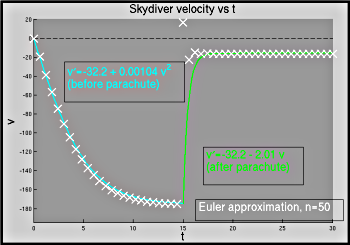
- Skydiver_Euler_Basic.m:
A very simple demo that steps shows the Euler approximation; it
graphs the exact solution and Euler approximation together.
[show
figure]
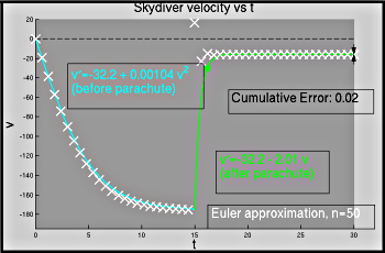
- Skydiver_Euler_Method.m:
A demo that steps shows the Euler approximation; with pauses, it
graphs first the exact solution, then the Euler approximation, then
the local error at a predefined time, and finally the cumulative
error.
[show
figure]
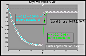
- Skydiver_Euler_Error.m:
A demo that steps shows the exact solution to the problem and the
Euler approximation; then, with pauses, it shows the local error at
a number of different points in the domain, and then finally the
cumulative error.
[show
figure]
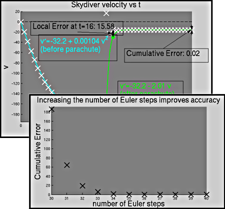
- Skydiver_Euler_Error_Cumulative.m:
A demonstration showing the exact solution and Euler approximation,
with the local and cumulative error, on one graph. After a pause,
it shows a second graph that shows how the cumulative error varies
with the number of steps used.
[show
figure]
Looking at the Model
Some questions that may be worth considering:
- How does the local error vary with the time in the simulation, and why?
- How can we predict the number of steps needed to obtain a given level of accuracy?
