Abstract
The standard model for a falling object with air resistance is adapted for a skydiver by including a piecewise air resistance term. The common models for air resistance are linear and quadratic; this model uses both, allowing the illustration of how both may be solved exactly. The resulting graph of the solution for the skydiver's velocity is a nice illustration of how the solutions fit together.
Use Cases
Lecture: Given the text's background on acceleration-velocity models, this model may be stated with minimal derivation. Solutions for both cases in the air resistance may be derived (with the initial condition for the second half being determined from the solution to the first half). The demonstrations simply graph the solution curves.
Outside of Lecture: Check that the forms of the two resistance terms make sense (that is, that the forces are in the correct direction). Assume that parachute deployment is at \(t=15\) and solve the initial value problem (this requires solving the first half and then using that solution to find the initial value at \(t=15\)). Graph your solution and verify that it matches the solution in these demonstrations.
Model Description
We model the velocity of a skydiver by considering her/his motion in two phases: before and after her/his parachute opens. In either case we have a first-order ordinary differential equation for the velocity, \[ \frac{dv}{dt} = -g + F_R, \] where \(g\) is the acceleration due to gravity and \(F_R\) is the force of air resistance divided by the mass of the skydiver. Note that here we take upwards to be the positive direction, so that the force of gravity pulls in the negative direction and \(F_R > 0\) opposes that motion.
Two common models for \(F_R\) are linear and quadratic resistances. For this demonstration we consider a quadratic resistance before the parachute opens and a linear resistance thereafter: \[ F_R = \begin{cases} k_1\,v^2 & \mbox{before deployment}\\ -k_2\,v & \mbox{after deployment}. \end{cases} \] It is worth observing that this is a different model than that used in most textbooks.
ODE Model
Using data from [1], we have that the terminal velocity of a parachuter in the USAF Academy Parachute Team (jumping from 4000 ft, or 1,219 m) is 120 mph (176 ft/s, or 53.6 m/s). Free-fall lasts about 10 sec, and free-falls over 13 sec are grounds for removal from the team. Landing velocity (which we take to the limiting velocity after parachute deployment) should be no worse than a fall from a 5 ft (1.52 m) wall, about 15-17 ft/s (4.6-5.2 m/s).
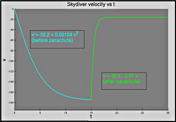
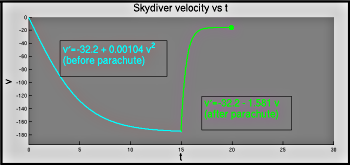
With \(g = 32.2\) ft/s and \(v_{T1} = 176\) ft/s, we have \(k_1 = 32.2/176^2 = 0.00104\). Similarly, with \(v_{T2} = 16\) ft/s, \(k_2 = 32.2/16 = 2.01\). Thus, in English units, we have the model \[ \frac{dv}{dt} = -32.2 + \begin{cases} 0.00104\,v^2 & \mbox{before deployment}\\ -2.01\,v & \mbox{after deployment} \end{cases}. \] We take \(v(0) = 0\), and (USAF Academy Parachute Team rules notwithstanding) that deployment occurs at \(t=15\).
We can solve this exactly, or numerically. It is worth noting that the discontinuous change in \(F_R\) results in a discontinuity in the acceleration experienced by the skydiver, which has negative ramifications for the structural integrity of her/his body (this resulting in an infinite force); this can be resolved by patching a smooth function between the two air resistances (though we do not include this in the model presented here). For details, see [1].
Matlab Demos
We consider a number of Matlab demos for this:
- Skydiver.m:
A very simple demo that graphs the (exact) solution to the
ODE.
[show
figure]
- Skydiver_Animated.m:
An animation of the solution, showing the \((t,v)\) point as a
function of \(t\).
[show
figure]
Looking at the Model
Some questions that may be worth considering:
- How does the modeled velocity change if we change the time at which the parachute opens?
- What does the graph of the distance fallen look like?
- What is the constraint on the opening time? How late could a parachuter open her/his parachute and still land safely? (This requires knowledge of the jump height and distance fallen.)
- Is the requirement that a parachuter's parachute be deployed in under 13 seconds a good one?
