Abstract
Our approach to population modeling is to take \(P' = \mbox{births} - \mbox{deaths}\). In this model we consider a situation in which a "non-standard" model for the deaths term is appropriate. The resulting differential equation is autonomous and first-order, and therefore separable, but separation does not provide useful information about solutions. The equation is amenable to numerical and qualitative analysis, however. These demonstrations show the numerical solutions to the system for different values of a parameter, and relate that to qualitative (phase line) analyses.
Use Cases
Lecture: The modeling equation can be used with a verbal description of why it has the form it does to illustrate how population models may vary. The numerical solutions provide both insight into why numerical methods are useful, and suggest the value of the qualitative analysis. The demonstrations looking at the qualitative analysis seek to motivate the phase line by looking at the behavior of solutions, the graph of the right-hand-side of the differential equation, and then the phase line.
Outside of Lecture: Look at each term in the differential equation and check that you can see where the terms in the logistic model appear, and what additional term is present. Convince yourself that it will do what we expect (it reflects predation: should it increase or decrease \(u'\)?). See how the solutions change as \(Q\) changes. For different values of \(Q\) sketch the phase line from the graphs of the right-hand side of the differential equation and see how it captures the long-term behavior of solutions to the differential equation.
Model Description
We model the population of the spruce budworm, which is an insect that is the most widely distributed and destructive defoliator of coniferous forests in Western North America[1]. Its population may be modeled by a logistic differential equation with the addition of a predation term. The latter term may reflect avian predation. The model used here is taken from Murray, Mathematical Biology[2].
ODE Model
Let \(u\) be a measure of the budworm population (in our model, it is a scaled population density). Then we can model \(u\) with \[ \frac{du}{dt} = r\,u\,(1 - \frac{u}{Q}) - \frac{u^2}{1 + u^2}, \] where \(r\) is a measure of the combined effects of the budworm birth rate, death rate and other population losses. \(Q\) is a carrying capacity, limiting the growth of the budworm population, and the term \(\frac{u^2}{1 + u^2}\) is a model for (avian) predation.
A crucial question (from the perspective of forest management) is whether the budworm population grows to "epidemic" levels—that is, levels at which significant amounts of forest will be defoliated. For the parameter values used here (which are not entirely representative of actual outbreak data; see, for example, [3]), we may take \( u > 4 \) as representing epidemic levels of infestation.
Matlab Demos
We consider a number of Matlab demos for this:
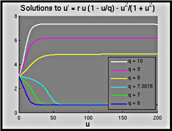
- Budworm_Model_Solution.m:
A very simple demo that numerically solves the ODE and plots the
solution for different values of \(Q\). The first graph is shown,
and then other values after a pause.
[show
figure]
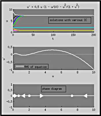
- Budworm_Phase_Plane.m:
Another simple demo that shows three graphs (with a pause between
each): the solution to the differential equation for a given value
of \(Q\), the corresponding graph of the right-hand side of the ODE
and resulting phase diagram, and the phase diagram itself.
[show
figure]
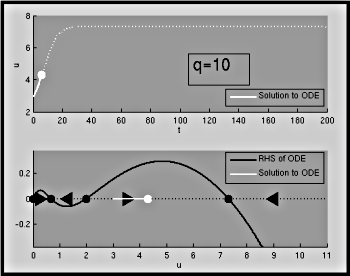
- Budworm_Animated_Phase_Plane.m:
A demonstration showing the graph of the solution and the phase line
at the same time (for given values of \(Q\) and \(r\)). These are
animated, showing a point \((t,u)\) on both graphs as time
increases (and therefore illustrating how time is implicit in the
graph of the phase line).
[show
figure]
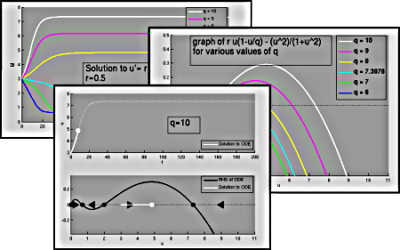
- Budworm_Model.m:
A demonstration that steps through all facets of the analysis of the
model. First graphs the solution curves for a set of interesting
values of \(Q\), then shows all of these together, then graphs the
right-hand side of the ODE for each of those values of \(Q\), and
finally animates the solution and phase diagram for a set of \(Q\)
values.
[show
figure]
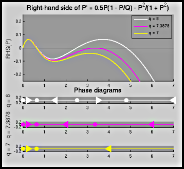
- Budworm_Bifurcation_Sequence.m:
A demonstration that shows the right-hand side of the differential
equation for three different values of \(Q\), one before, one at and
one after the bifurcation point where one and then two larger
equilibrium solutions come into being. Then phase diagrams for the
three cases are shown, which (if turned around to reverse the \(x\)-
and \(y\)-axes) become a bifurcation diagram.
[show
figure]
Looking at the Model
Some questions that may be worth considering:
- What initial conditions result in a non-epidemic population of budworms?
- How is this influenced by the value of the carrying capacity \(Q\)?
- What is special about the value \(Q = 7.3878\) of the carrying capacity? What implication does this have for the management of the budworm population?
- Note that \(Q\) can be changed by applying insecticide to the fir trees on which the budworm lives. However, in some areas (or in some contexts) it may not be desirable to use insecticide in this manner. Suppose that we change the growth rate \(r\) (for example, by introducing budworm-specific diseases or sterile budworms into the population). Can we use this to produce non-epidemic populations of budworms?
References
- Fellin, D. and J. Dewey (March 1992). Western Spruce Budworm Forest Insect & Disease Leaflet 53, U.S. Forest Service. Retrieved on: 9 Aug, 2012.
- Murray, J.D. Mathematical Biology, 3rd ed. New York:Springer, 2002.
- Ludwig, D., Jones, D.D., and C.S. Holling. Qualitative Analysis of Insect Outbreak Systems: The Spruce Budworm and Forest. J. Anim. Ecol. 47, 315-332 (1978).
