Math 215 Examples

Key Concepts

Line Integrals with respect to Arc Length

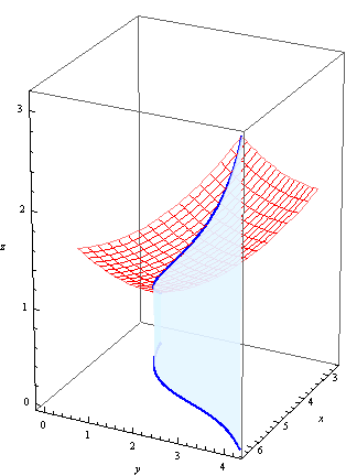
Let \(C\) be a curve in the \(xy\)-plane, and let \(f(x,y)\) be a function. Then the line integral of \(f\) along \(C\) is denoted \(\int_C f(x,y)\, ds\) and is equal to the signed area between the surface \(z=f(x,y)\) and the curve \(C\):

We sometimes call this the line integral with respect to arc length to distinguish from two other kinds of line integrals that we will discuss soon.

Riemann Sums for Line Integrals

As usual, to give a formal symbolic definition of an integral, we think of it as a limit of Riemann sums. We can approximate the area with rectangles whose bases follow the curve \(C\) and whose heights are values of the function \(f(x,y)\). As usual, as we use more and more rectangles, the Riemann sum approximates the area more and more closely:

How can we use this to write down a limit definition for line integrals? Suppose that our curve \(C\) is parameterized by \((x(t),y(t))\) for \(a\le t\le b\). Now divide our interval into \(n\) subintervals with endpoints \(a = t_0 \lt t_1 \lt t_2 \lt \dots \lt t_n = b\), and pick sample points \(t^*_i \in [t_{i-1},t_i]\). The \(i\)th subinterval \([t_{i-1},t_i]\) corresponds to the rectangle whose base are the two points along the curve \((x(t_{i-1}),y(t_{i-1}))\) and \((x(t_i),y(t_i))\) with height \(f(x(t^*_i),y(t^*_i))\). The base has length \[ \sqrt{(x(t_i)-x(t_{i-1}))^2 + (y(t_i)-y(t_{i-1}))^2}, \] which we can write as \[ \sqrt{(\Delta x_i)^2 + (\Delta y_i^2)}. \] Then the sum of the areas of the rectangles is \[ \int_C f(x,y)\, ds \approx \sum_{i=1}^n f(x(t^*_i), y(t^*_i))\sqrt{(\Delta x_i)^2 + (\Delta y_i)^2}. \] This yields the following definition:

Computing Line Integrals Symbolically

We can use this limit definition to rewrite the line integral as a single-variable integral. Note that we can rewrite the square root as \[ \sqrt{(\Delta x_i)^2 + (\Delta y_i)^2}\ = \Delta t\sqrt{\left(\frac{\Delta x_i}{\Delta t}\right)^2 + \left(\frac{\Delta y_i}{\Delta t}\right)^2}. \] In the limit as \(n\to\infty\), \(\frac{\Delta x_i}{\Delta t}\to x'(t^*_i)\) and \(\frac{\Delta y_i}{\Delta t}\to y'(t^*_i)\), so we have \[\begin{aligned} \lim_{n\to\infty}\sum_{i=1}^n f(x(t^*_i), y(t^*_i))\sqrt{(\Delta x_i)^2 + (\Delta y_i)^2} &= \lim_{n\to\infty}\sum_{i=1}^n f(x(t^*_i), y(t^*_i)) \sqrt{x'(t^*_i)^2 + y'(t^*_i)^2} \Delta t \\ &= \int_a^b f(x(t),y(t))\sqrt{x'(t)^2+y'(t)^2}\, dt. \end{aligned}\] We therefore have

Line Integrals with respect to \(x\) and \(y\)

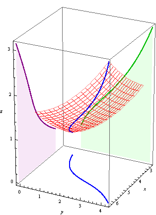
Occasionally, we will instead wish to integrate with respect to \(x\) or \(y\), rather than with respect to arclength. The line integral \(\int_C f(x,y)\, dx\) corresponds to the area under the projection of the curve onto the \(xz\)-plane, and similarly \(\int_C f(x,y)\, dy\) to the projection to the \(yz\)-plane:

We can compute Riemann sums for these similarly, leading to the following formulas:

Illustrated Example

Worked Solution

First, let us parameterize \(C\) as \((2\cos t, 2\sin t)\) for \(0\le t \le \pi\). We will use a Riemann sum with three equal subdivisions, with sample points in the middle of each subdivision. Our three \(t\)-subintervals are \([0,\pi/3]\) with sample point \(t=\pi/6\), \([\pi/3,2\pi/3]\) with sample point \(t=\pi/2\), and \([2\pi/3,\pi]\) with sample point \(t=5\pi/6\).

The base of the first rectangle is between \((2\cos 0,2\sin 0) = (2,0)\) and \((2\cos\frac{\pi}{3},2\sin\frac{\pi}{3}) = (1,\sqrt{3})\), with length \(\sqrt{(1-2)^2+(\sqrt{3}-0)^2} = \sqrt{1+3} = 2\). The height of this rectangle is the value of the function at \((x(\pi/6),y(\pi/6)) = (\sqrt{3},1)\), or \(f(\sqrt{3},1) = 3-1+3 = 5\). The area of this rectangle, then, is \(2\cdot 5 = 10\).

The base of the second rectangle is between \((2\cos\frac{\pi}{3},2\sin\frac{\pi}{3}) = (1,\sqrt{3})\) and \((2\cos \frac{2\pi}{3},2\sin \frac{2\pi}{3}) = (-1,\sqrt{3})\), with length \(\sqrt{(-1-1)^2+(\sqrt{3}-\sqrt{3})^2} = \sqrt{4+0} = 2\). The height of this rectangle is the value of the function at \((x(\pi/2),y(\pi/2)) = (0,2)\), or \(f(0,2) = 0-2+3 = 1\). The area of this rectangle, then, is \(2\cdot 1 = 2\).

The base of the third and last rectangle is between \((2\cos\frac{2\pi}{3},2\sin\frac{2\pi}{3}) = (-1,\sqrt{3})\) and \((2\cos\pi, 2\sin\pi) = (-2,0)\), with length \(\sqrt{(-2+1)^2+(0-\sqrt{3})^2} = \sqrt{1+3} = 2\). The height of this rectangle is the value of the function at \((x(5\pi/6),y(5\pi/6)) = (-\sqrt{3},1)\), or \(f(-\sqrt{3},1) = 3-1+3 = 5\). The area of this rectangle, then, is \(2\cdot 5 = 10\).

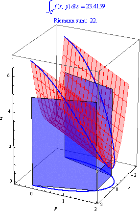
In total, then, the Riemann sum gives \[ \int_C f(x,y)\, dx \approx 10 + 2 + 10 = 22. \]

To compute this exactly, we find \(x'(t) = -2\sin t\) and \(y'(t) = 2\cos t\), so that \[ \sqrt{x'(t)^2 + y'(t)^2} = \sqrt{4\sin^2 t + 4\cos^2 t} = \sqrt{4} = 2. \] Hence \[\begin{aligned} \int_C f(x,y)\, dx &= \int_0^\pi f(2\cos t, 2\sin t) \sqrt{x'(t)^2+y'(t)^2}\, dt \\ &= \int_0^\pi (4\cos^2 t - 2\sin t + 3) \cdot 2\, dt. \end{aligned}\] By using the double angle formula from trigonometry, we can write \(4\cos^2 t = 2\cos(2t) + 2\), so that the integrand becomes \[ (2\cos(2t)-2\sin t+5)\cdot 2 = 4\cos(2t)-4\sin t+10. \] This has as an antiderivative \(2\sin(2t)+4\cos t+10t\), and hence we conclude \[ \int_C f(x,y)\, dx = (2\sin(2t)+4\cos t+10t)\big|_0^\pi = (0-4+10\pi)-(0+4+0) = 10\pi - 8. \]

Note that \(10\pi -8 \approx 23.4\), so our estimate of \(22\) with just \(3\) rectangles was not too bad.

Visualizing the Example

The image below shows the rectangle corresponding to this Riemann sum:

Further Questions

1. We could have known ahead of time that the area of the third rectangle in the Riemann sum would equal the area of the first rectangle. Explain how.
2. Use the idea from Question 1 to do a Riemann sum with \(2\) subdivisions with minimal calculation.
3. Would the argument from Question 1 still work if \(f(x,y) = x - y^2+3\) instead? What if we kept \(f(x,y) = x^2 - y+3\), but changed \(C\) to be the semicircle lying to the right of the \(y\)-axis? What if we changed both, to \(f(x,y) = x - y^2 + 3\) and \(C\) as the semicircle right of the \(y\)-axis?
4. Compute the exact values of \(\int_C f(x,y)\, dx\) and \(\int_C f(x,y)\, dy\) with \(f(x,y)\) and \(C\) as in the example.

Using the Mathematica Demo

All graphics on this page were generated by the Mathematica notebook 16_2LineIntegrals.nb.

This notebook generates images and animations like those on this page for any function and curve.

As an exercise, use the notebook to provide visual demonstration illustrating your answers to Questions 2-4.

The notebook also allows you to specify where in each subinterval to pick the sample point. What happens if we always take the left endpoint as a sample point? What about the right end point? Use the notebook to investigate how quickly the Riemann sums converge for different sample points.