Math 215 Examples

Key Concepts

Regions of Type I and II

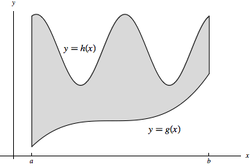
A region in the \(xy\)-plane is called type I if it is defined as the region between two functions of \(x\):

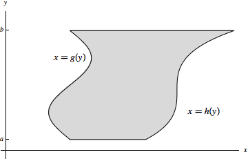
A region in the \(xy\)-plane is called type II if it is defined as the region between two functions of \(y\):

Integrating over Regions of Type I

To visualize this, imagine the slice at a fixed value of \(x\). This slice begins at \(g(x)\) and ends at \(h(x)\). Shown below-left is the region in the \(xy\)-plane, with the slice drawn as a blue arrow, and below-right is the slice drawn in a 3D-coordinate system. (Note that the origin in the 3D-coordinate system is at the bottom right of the box.)

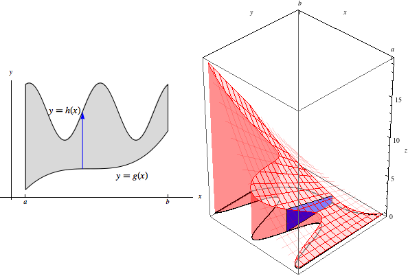
The area under this slice is \[\text{Area}(x)=\int_{g(x)}^{h(x)} f(x,y)\, dy.\] As with rectangular regions, then, to compute the original double integral, we sweep through the entire volume as these slices range from \(x=a\) to \(x=b\):

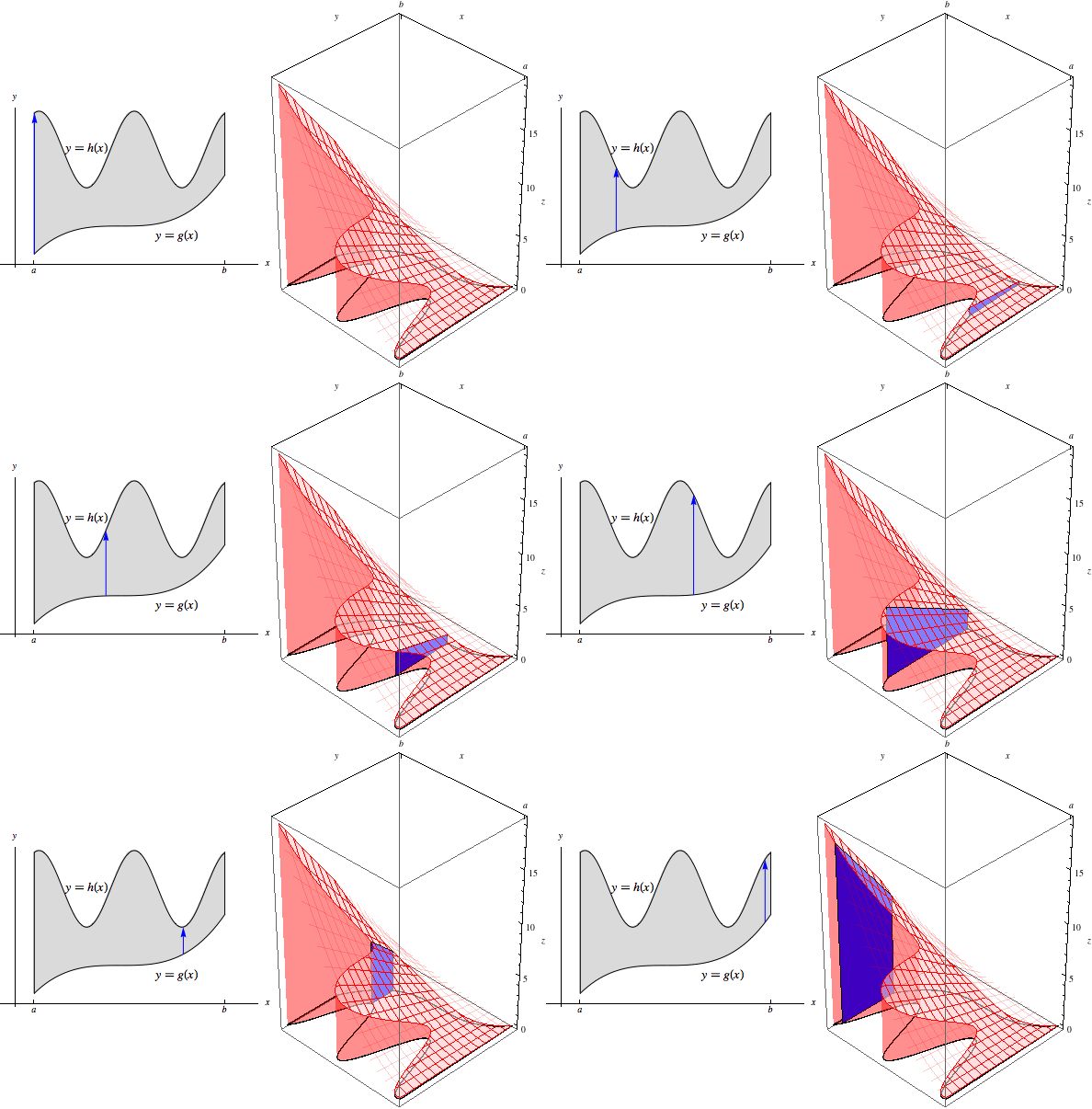
This yields the final result of \[\iint\limits_R f(x,y)\, dA = \int_a^b \text{Area}(x)\, dx = \int_a^b\int_{g(x)}^{h(x)} f(x,y)\, dy\, dx.\]

Integrating over Regions of Type II

This situation is analogous to the one above for type I regions, but now our slices are at fixed \(y\)-values. The slice at \(y\) begins at \(g(y)\) and ends at \(h(y)\):

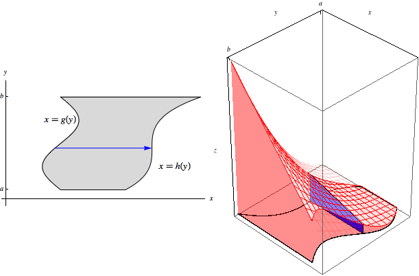
The area under this slice is \[\text{Area}(y)=\int_{g(y)}^{h(y)} f(x,y)\, dx.\] As these slices of area range through from \(y=a\) to \(y=b\), we sweep through the entire volume:

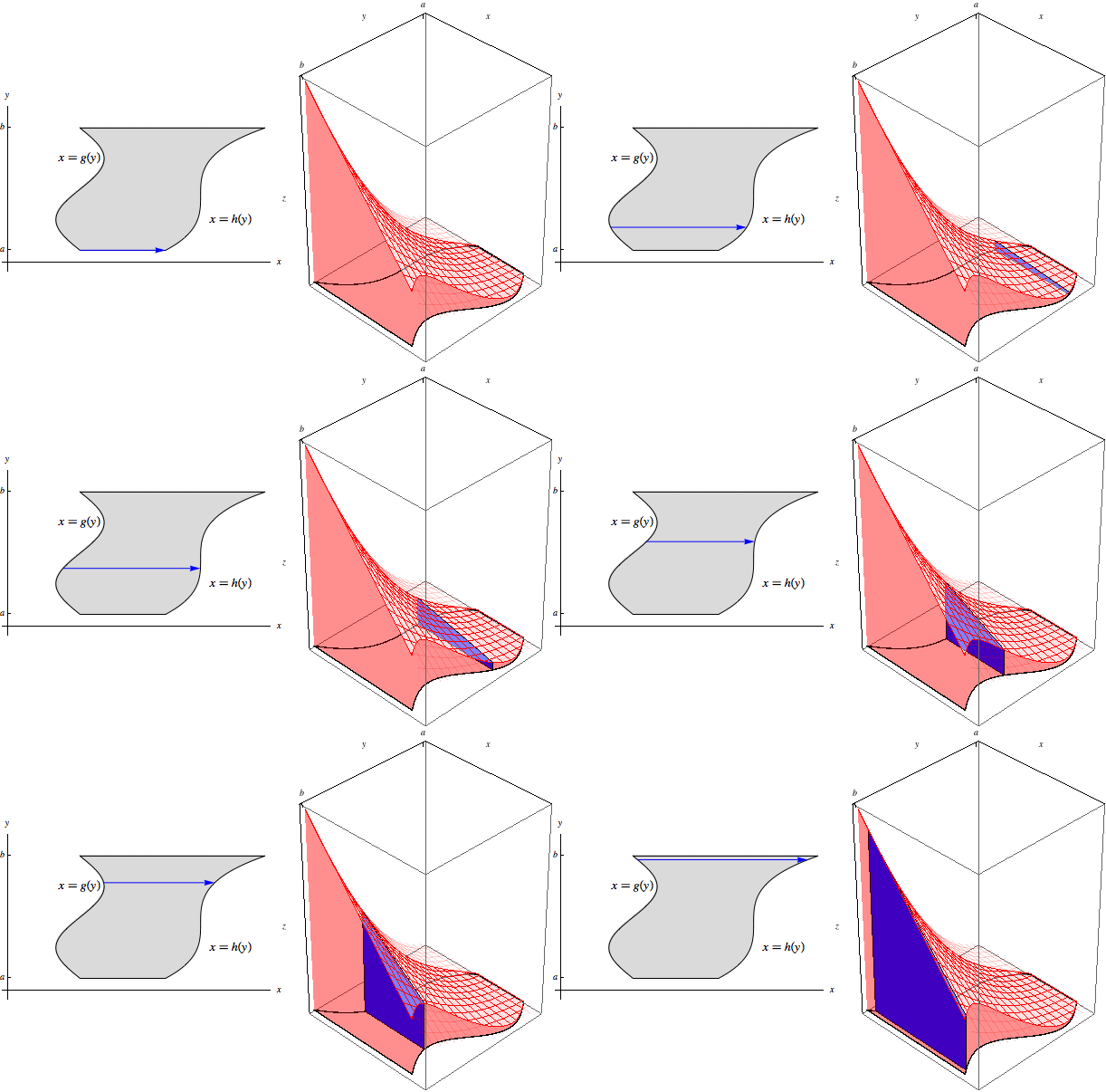
Hence \[\iint\limits_R f(x,y)\, dA = \int_a^b \text{Area}(y)\, dy = \int_a^b\int_{g(y)}^{h(y)} f(x,y)\, dx\, dy.\]

Illustrated Example

Worked Solution

Let us first look at this region \(R\) in the \(xy\)-plane:

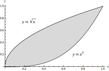
The intersection points occur when \(x^3=\sqrt{x}\), which we can solve to find \(x=0\) and \(x=1\). Notice that for \(0\le x\le 1\), the curve \(y=\sqrt{x}\) is on top and \(y=x^3\) is on the bottom. Hence \(R\) is the type I region defined by \(0\le x\le 1\) and \(x^3\le y\le \sqrt{x}\).

We can now write the desired double integral as an iterated integral: \[\iint\limits_R x^2 y\, dA = \int_0^1\int_{x^3}^{\sqrt{x}} x^2 y\, dy\, dx\] We evaluate the inner integral treating \(x\) as constant: \[\begin{aligned}\int_{x^3}^{\sqrt{x}} x^2 y\, dy &= \frac{1}{2}x^2y^2 \Big|_{x^3}^{\sqrt{x}} \\ &= \frac{1}{2}(x^3-x^8) \end{aligned}\]

Using this, we have \[\begin{aligned} \iint\limits_R x^2 y\, dA &= \int_0^1\int_{x^3}^{\sqrt{x}} x^2 y\, dy\, dx \\ &= \int_0^1 \frac{1}{2}(x^3-x^8)\, dx \\ &= (x^4/8 - x^9/18) \Big|_0^1 \\ &= (1/8-1/18)-(0-0) = 5/72. \end{aligned}\]

Visualizing the Example

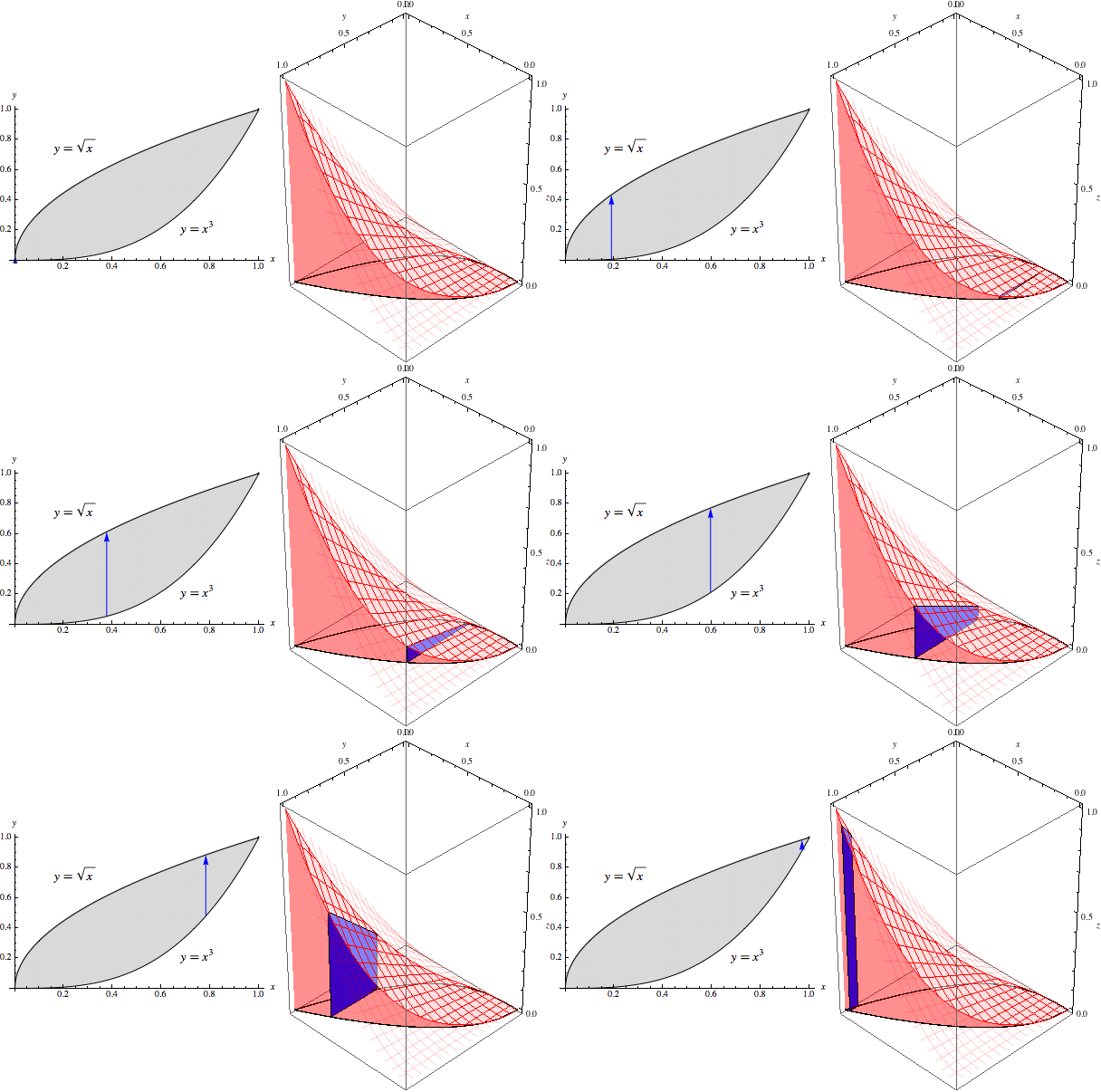
Our inner integral \(\int_{x^3}^{\sqrt{x}} x^2y\, dy\) gives the area of the slice at any \(x\) value. For example, at \(x=0.6\), we have the slice shown below.

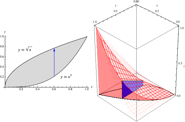
Plugging \(x=0.6\) into this integral, we see that the area of this slice is \[\begin{aligned} \int_{0.6^3}^{\sqrt{0.6}} 0.6^2y\, dy &= \int_{0.216}^{\sqrt{0.6}} 0.36y\, dy \\ &= 0.18y^2\Big|_{0.216}^{\sqrt{0.6}} \\ &= 0.18(0.6 - 0.216^2) = 0.0996. \end{aligned}\] Note that this is exactly what we get when we plug \(x=0.6\) into \(\frac{1}{2}(x^3-x^8)\), as we computed in general that \[\int_{x^3}^{\sqrt{x}} x^2y\, dy = \frac{1}{2}(x^3-x^8).\]

As we let \(x\) range from \(0\) to \(1\), these slices sweep out the entire volume of \(5/72\):

Further Questions

1. What is the area under the slice at \(x=0.4\)? What is the area under the slice at \(x=1\)?
2. Suppose we switched the bounds on the inner integral and instead integrated from \(\sqrt{x}\) to \(x^3\). How would this mistake affect the final answer?
3. The region \(R\) in the example is also a type II region. What functions \(x=g(y)\) and \(x=h(y)\) bound it?
4. Evaluate the integral in the example by treating \(R\) as the type II region you described in Question 3.

Using the Mathematica Demo

All graphics on this page were generated by the Mathematica notebook 15_3DoubleIntegralsOverGeneralRegions.

This notebook generates images and animations like those on this page for any type I region with \(y=g(x)\) and \(y=h(x)\). The notebook also provides many additional options, including the option to attempt to treat the region as type II.

As an exercise, use the notebook to provide a clear graphical answer to Question 3. You can do this simply by setting regionType = 2 and re-executing the code in the Graphics section. Then feel free to change the bounds and the function \(f(x,y)\) itself, keeping in mind the limitations described in the notebook.