Key Concepts
Definition of a Double Integral
We can if we wish consistently choose our sample points.
If we always choose the top right corner of each subrectangle, then we see \[\iint\limits_R f(x,y)\, dA = \lim_{m,n\to\infty} \sum_{i=1}^m\sum_{j=1}^n f(x_i,y_j)\Delta A.\]
If we always choose the bottom left corner, then we have instead \[\iint\limits_R f(x,y)\, dA = \lim_{m,n\to\infty} \sum_{i=0}^{m-1}\sum_{j=0}^{n-1} f(x_i,y_j)\Delta A\] (notice the bounds on the sums!).
Finally, as is often the most useful for approximations, if we choose the midpoint \((\bar{x_i},\bar{y_j})\) of each subrectangle, then we have \[\iint\limits_R f(x,y)\, dA = \lim_{m,n\to\infty} \sum_{i=1}^m\sum_{j=1}^n f(\bar x_i,\bar y_j)\Delta A.\]
When the double integral exists at all, all three of these formulas will give the same result.
Double Riemann Sums
As with single-variable integrals, we can approximate double integrals by actually computing these double sums for a finite number of subrectangles (i.e., for finite \(m\) and \(n\)). Just as in the single-variable case, increasing the number of subrectangles improves our estimate. Notice that since we are dividing the \(x\)-interval into \(m\) subintervals and the \(y\)-interval into \(n\) subintervals, we in fact divide the entire rectangle \(R\) into \(mn\) rectangles.
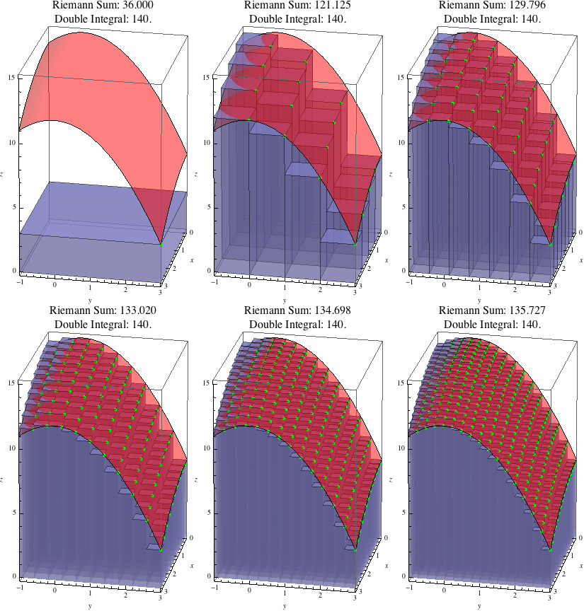
The animation below shows Riemann sums estimating \(\iint\limits_R (15-x^2/3-y^2)\, dA\) where \(R=[0,3]\times[-1,3]\). The animation begins with one rectangle (\(m=n=1\)) and ends with 256 subrectangles (\(m=n=16\)).

We can see that as the number of subrectangles increases, the boxes more closely approximate the actual function, and the Riemann sum more closely approximates the value of the double integral.
Illustrated Example
Worked Solution
Since we want \(0.5\times 0.5\) subrectangles, we will need to divide the \(x\) interval of \([1,2]\) into \(m=(2-1)/0.5=2\) subintervals each of width \(0.5\), and we similarly need to divide the \(y\) interval of \([0,2]\) into \(n=(2-0)/0.5=4\) subintervals each of width \(0.5\). Our \(x\) subintervals, then, are \([1,1.5]\) and \([1.5,2]\), with midpoints \(\bar x_1=1.25\) and \(\bar x_2=1.75\). Similarly, our \(y\) subintervals are \([0,0.5]\), \([0.5,1]\), \([1,1.5]\), and \([1.5,2]\), with midpoints \(\bar y_1=0.25\), \(\bar y_2=0.75\), \(\bar y_3=1.25\), and \(\bar y_4=1.75\).
The area of each subrectangle is \(\Delta A = 0.5\cdot 0.5=0.25\).
Putting this together, we have \[\begin{aligned} \iint\limits_R (3-x)(3-y)^2\, dA \approx & \sum_{i=1}^2\sum_{j=1}^4 (3-\bar x_i)(3-\bar y_j)^2\cdot 0.25 \\ \approx & 13.23\cdot0.25+8.86\cdot0.25+5.36\cdot0.25+2.73\cdot0.25+ 9.45\cdot0.25+6.33\cdot0.25+3.83\cdot0.25+1.95\cdot0.25 \\ \approx & 12.9. \end{aligned}\]
Visualizing the Example
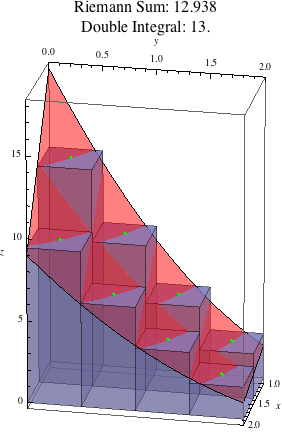
Shown below are the boxes for this Riemann sum:

Because we are doing a midpoint sum, the midpoints of the top of each box (shown by the green dots) lie on the graph of the function \(f(x,y)=(3-x)(3-y)^2\).
The heights of these green dots are the values \(13.23\), \(8.86\), \(5.36\), etc. showing up in the Riemann sum.
Since the base of each box has area \(\Delta A = 0.5\cdot 0.5=0.25\), the volume of the boxes, then, are \(13.23\cdot 0.25\), \(8.86\cdot 0.25\), \(5.36\cdot 0.25\), etc., which are precisely the terms of the Riemann sum.
Further Questions
- In the example above, we used \(m=2\) subdivisions of the \(x\)-interval and \(n=4\) subdivisions of the \(y\)-interval. How would the Riemann sum change if we instead used \(m=4\) subdivisions of the \(x\)-interval and \(n=2\) subdivisions of the \(y\)-interval?
- In general (i.e., for any Riemann sum approximating any double integral over any rectangle \(R\)), what is the relationship between the area of \(R\), the area of each subrectangle \(\Delta A\), the number of \(x\)-subdivisions \(m\), and the number of \(y\)-subdivisions \(n\)?
- For what sorts of functions is a Riemann sum with top right sample points
guaranteed to give an overestimate of the corresponding double integral?
When must it give an underestimate?
What about Riemann sums with bottom left sample points,
or top right sample points, or bottom right sample points?
(It may be helpful to think first about facts like why, in single-variable calculus, left Riemann sums of increasing functions are guaranteed to give underestimates of the corresponding definite integral.)
Using the Mathematica Demo
All graphics on this page were generated by the Mathematica notebook 15_1DoubleIntegralsOverRectangles.nb.
This notebook generates images and animations like those on this page for any integrand \(f(x,y)\) and any rectangle \(R\), as well as any choice of subdivision and any consistent way of choosing sample points.
As an exercise, use the notebook to provide visual examples illustrating your answers to Question 3.
Additionally, investigate how the choice of sample points affects the Riemann sum.
Suppose, say, that we were to redo the example, but with top right sample points
instead of midpoints.
Use the notebook to demonstrate this new Riemann sum visually.
Is the estimate better, worse, or about the same as the midpoint estimate?
What if we use \(4\) \(x\)-subdivisions and \(8\) \(y\)-subdivisions
with our top right sample points?
How many subdivisions do we need until the top right Riemann sum
provides an estimate as good as the midpoint Riemann sum from the example?
(You may be surprised by how many you need -- midpoint Riemann sums often
converge to the value of the double integral significantly faster!)