Math 215 Examples

Key Concepts

Constrained Extrema

Often, rather than finding the local or global extrema of a function, we wish to find extrema subject to an additional constraint. For example, we may wish to find the largest and smallest values a function \(f(x,y)\) achieves on the unit circle \(x^2+y^2=1\):

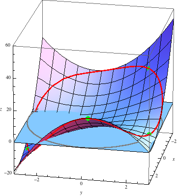
In this picture, the blue plane is the \(xy\)-plane, with the unit circle drawn on it in gray. The points of the graph of \(z=f(x,y)\) lying above the unit circle are drawn in red. In this picture, \(f(x,y)\) restricted to the unit circle has four local extrema, which are highlighted in green. (One of them is hard to see, but it's near the bottom right corner of the surface.)

Notice that even though these four points are local extrema of the constrained function, none of them are actually local extrema of \(f(x,y)\) when unconstrained! So finding critical points of \(f(x,y)\) will not help us find these points.

Once we have these points, however, finding the absolute maximum and minimum of \(f(x,y)\) subject to the constraint is straightforward: each absolute extremum must be at one of these points, so we simply plug these points into \(f(x,y)\) and pick out the largest and smallest values.

Lagrange Multipliers

To find these points, we use the method of Lagrange multipliers:

Why does this condition on the gradients of \(f(x,y)\) and \(g(x,y)\) relate to constrained extrema at all? Let \(M\) be the maximum value of \(f(x,y)\) subject to the constraint \(g(x,y)=0\). Think about the level curve \(f(x,y)=M\). Since \(f(x,y)\) achieves the value \(M\) somewhere on the constraint \(g(x,y)=0\), this level curve and \(g(x,y)=0\) must intersect. Now suppose we look the level curve \(f(x,y)=N\) for some N slightly bigger than M. This new level curve cannot intersect \(g(x,y)=0\), as by definition, \(M\) is the maximum value achieved by \(f(x,y)\) on \(g(x,y)=0\). Therefore, moving the level curve \(f(x,y)=M\) even slightly will cause it no longer to intersect \(g(x,y)=0\). This implies that \(f(x,y)=M\) and \(g(x,y)=0\) must in fact be tangent to each other.

For two curves in the plane to be tangent at a point, their normal vectors at that point must be parallel. But recall that the gradient vector at a point is always normal to the level curve through that point. So the fact that the level curves \(f(x,y)=M\) and \(g(x,y)=0\) are tangent at some point implies that the gradients of \(f(x,y)\) and \(g(x,y)\) are parallel at that point.

The following animation demonstrates this graphically, for the example surface graphed above. The constraint \(g(x,y)=0\) is drawn in red on top of the contour plot of the surface \(z=f(x,y)\). We then sweep through the level curves of \(z=f(x,y)\), starting at the bottom, corresponding to the darkest portions of the contour plot.

The first time a level curve touches the constraint is our constrained minimum. The level curve at this point is tangent to the constraint. The next two times the level curve is tangent to the constraint provide local extrema, and the final time gives us our constrained global maximum.

Illustrated Example

Worked Solution

Set \(f(x,y)=y^2-x\) and \(g(x,y)=2x^2+2xy+y^2-1\) so that our goal is to maximize \(f(x,y)\) subject to \(g(x,y)=0\).

By the method of Lagrange multipliers, we need to find simultaneous solutions to \[\nabla f(x,y) = \lambda\,\nabla g(x,y)\] and \[g(x,y)=0.\] We compute \[\nabla f(x,y) = \langle -1, 2y\rangle\] and \[\nabla g(x,y) = \langle 4x+2y, 2x+2y\rangle.\] The vector equality \[\langle -1, 2y\rangle\ = \lambda\,\langle 4x+2y, 2x+2y\rangle\] is equivalent to the coordinate-wise equalities \[\begin{aligned} -1 &= \lambda(4x+2y) \\ 2y &= \lambda(2x+2y). \end{aligned}\]

Solving for \(\lambda\) in each equation gives \[\begin{aligned} \lambda &= \frac{-1}{4x+2y} \\ \lambda &= \frac{y}{x+y}. \end{aligned}\] Since \(\lambda\) must take on a consistent value throughout, the two right-hand sides of the above equations must be equal, and we can use this to solve for \(x\) in terms of \(y\): \[\begin{aligned} \frac{y}{x+y} &= \frac{-1}{4x+2y} \\ y(4x+2y) &= -(x+y) \\ 4xy+2y^2 &= -x-y \\ 4xy+x &= -(2y^2+y) \\ x(4y+1) &= -(2y^2+y) \\ x &= -\frac{2y^2+y}{4y+1}. \end{aligned}\]

We must also satisfy the constraint \(g(x,y)=0\), so plugging this in, we need \[\begin{aligned} g(x,y) &= 0 \\ 2x^2+2xy+y^2-1 &= 0 \\ 2\frac{(2y^2+y)^2}{(4y+1)^2}-2\frac{2y^3+y^2}{4y+1}+y^2-1 &= 0. \end{aligned}\]

At this point, we have reduced the problem to solving for the roots of a single variable polynomial, which any standard graphing calculator or computer algebra system can solve for us, yielding the four solutions \[ y\approx -1.38,-0.31,-0.21,1.40. \]

Plugging these back in to \(x = -\frac{2y^2+y}{4y+1}\) gives the corresponding \(x\)-values of approximately \(0.54,-0.54,0.81,-0.81\). Our four candidates for the constrained global extrema, then, are the points \((0.54,-1.38),(-0.54,-0.31),(0.81,-0.21),(-0.81,1.40)\). To figure out which one is the global maximum we were asked for, we simply plug them all into \(f(x,y)\): \[\begin{aligned} f(0.54,-1.38) &\approx 1.37 \\ f(-0.54,-0.31) &\approx 0.63 \\ f(0.81,-0.21) &\approx -0.76 \\ f(-0.81,1.40) &\approx 2.76. \end{aligned}\]

We conclude that the maximum value of \(f(x,y)=y^2-x\) subject to the constraint \(g(x,y)=2x^2+2xy+y^2-1=0\) is \(2.76\), occurring at the point \((-0.81,1.40)\).

Visualizing the Example

Shown below is the graph of \(z=y^2-x\) with the constraint \(2x^2+2xy+y^2=1\) drawn on it in red.

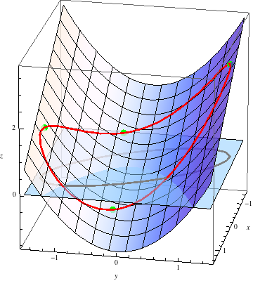
The constrained maximum clearly occurs at the green point near the top right of the image. While it is hard to read precise coordinates off of a 3-dimensional plot, it looks like this point occurs at an \(x\)-value between \(-1\) and \(0\), and a \(y\)-value bigger than \(1\), and the value of \(y^2-x\) here appears to be somewhat larger than \(2\). All these observations agree with the coordinates of this maximum that we calculated of \((-0.81,1.40,2.76)\).

Further Questions

1. The method of Lagrange multipliers in this example gave us four candidates for the constrained global extrema. We discussed where the global maximum appears on the graph above. Find the other three candidates on the graph. Which is the constrained global minimum?
2. You may have noticed that the \(x\)-values in the example came in pairs: \(x=\pm 0.54\) and \(x=\pm 0.81\). This suggests that if
3. Do constrained global extrema always exist? Can you give an example of a function \(f(x,y)\) and a constraint \(g(x,y)=0\) such that \(f(x,y)\) has a constrained global maximum but no constrained global minimum?
4. In all of the images on this page, all of the candidate global extrema provided by the method of Lagrange multipliers are at least constrained local extrema. Can you give an example of a function \(f(x,y)\) and a constraint \(g(x,y)=0\) such that at least one of the candidates provided by the method of Lagrange multipliers is not even a constrained local extremum?

Using the Mathematica Demo

All graphics on this page were generated by the Mathematica notebook 14_8Lagrange_Multipliers.nb.